
Gaussian Processes Explained: A Visual Introduction
Introduction to Gaussian Processes
Gaussian Processes (GPs) are a powerful and elegant approach to machine learning that provide a principled, practical, and probabilistic approach to learning in kernel machines. They define a distribution over functions which can be used for Bayesian regression, classification and other tasks.
The Mathematics Behind Gaussian Processes
At the heart of Gaussian Processes is the multivariate Gaussian distribution. A Gaussian Process is a collection of random variables, any finite number of which have a joint Gaussian distribution. A GP is completely specified by its mean function and covariance function .
import numpy as np
from sklearn.gaussian_process import GaussianProcessRegressor
from sklearn.gaussian_process.kernels import RBF

# Define the kernel
kernel = 1.0 * RBF(length_scale=1.0)

# Create GP regressor
gp = GaussianProcessRegressor(kernel=kernel, n_restarts_optimizer=10)

# Generate sample data
X = np.linspace(0, 5, 10).reshape(-1, 1)
y = np.sin(X).ravel() + 0.1 * np.random.randn(10)

# Fit the model
gp.fit(X, y)

Applications in Machine Learning
Gaussian Processes are particularly useful for regression problems, optimization, and in active learning scenarios. They provide not just predictions but also uncertainty estimates, which is crucial in many applications.

Gaussian Process Visualization

Implementation Example
Here's how you might implement a simple GP regression in Python using scikit-learn:

Choose an appropriate kernel
Create a GP regressor
Fit the model to your data
Make predictions with uncertainty estimates
# Plot the results
X_test = np.linspace(0, 5, 100).reshape(-1, 1)
y_pred, y_std = gp.predict(X_test, return_std=True)

import matplotlib.pyplot as plt
plt.figure(figsize=(10, 6))
plt.plot(X, y, 'r.', markersize=10, label='Observations')
plt.plot(X_test, y_pred, 'b-', label='Prediction')
plt.fill_between(X_test.ravel(),
         y_pred - 1.96 * y_std,
         y_pred + 1.96 * y_std,
         alpha=0.2, color='blue',
         label='95% confidence interval')
plt.xlabel('x')
plt.ylabel('f(x)')
plt.legend()
plt.title('Gaussian Process Regression')
plt.grid(True)
Advantages of Gaussian Processes
- Uncertainty Quantification: GPs provide a principled way to quantify uncertainty in predictions.
- Flexibility: They can model a wide variety of functions by choosing appropriate kernels.
- Interpretability: The hyperparameters of the kernel have interpretable meanings.
- Small Data Performance: GPs can perform well even with relatively small datasets.
Limitations and Challenges
Despite their elegance, Gaussian Processes face some challenges:
- Computational Complexity: Standard GP implementations scale as O(n³) with the number of data points.
- High Dimensions: They can struggle in very high-dimensional spaces (the "curse of dimensionality").
- Hyperparameter Selection: Choosing appropriate kernel hyperparameters can be challenging.
Conclusion
Gaussian Processes offer a powerful framework for probabilistic modeling with built-in uncertainty estimation. Their mathematical elegance combined with practical utility makes them an essential tool in the modern machine learning toolkit, particularly for problems where quantifying uncertainty is important.
Related Posts
More content from the Machine Learning category and similar topics

A comprehensive tutorial on understanding Gaussian Processes with interactive visualizations and practical examples.
Shared topics:
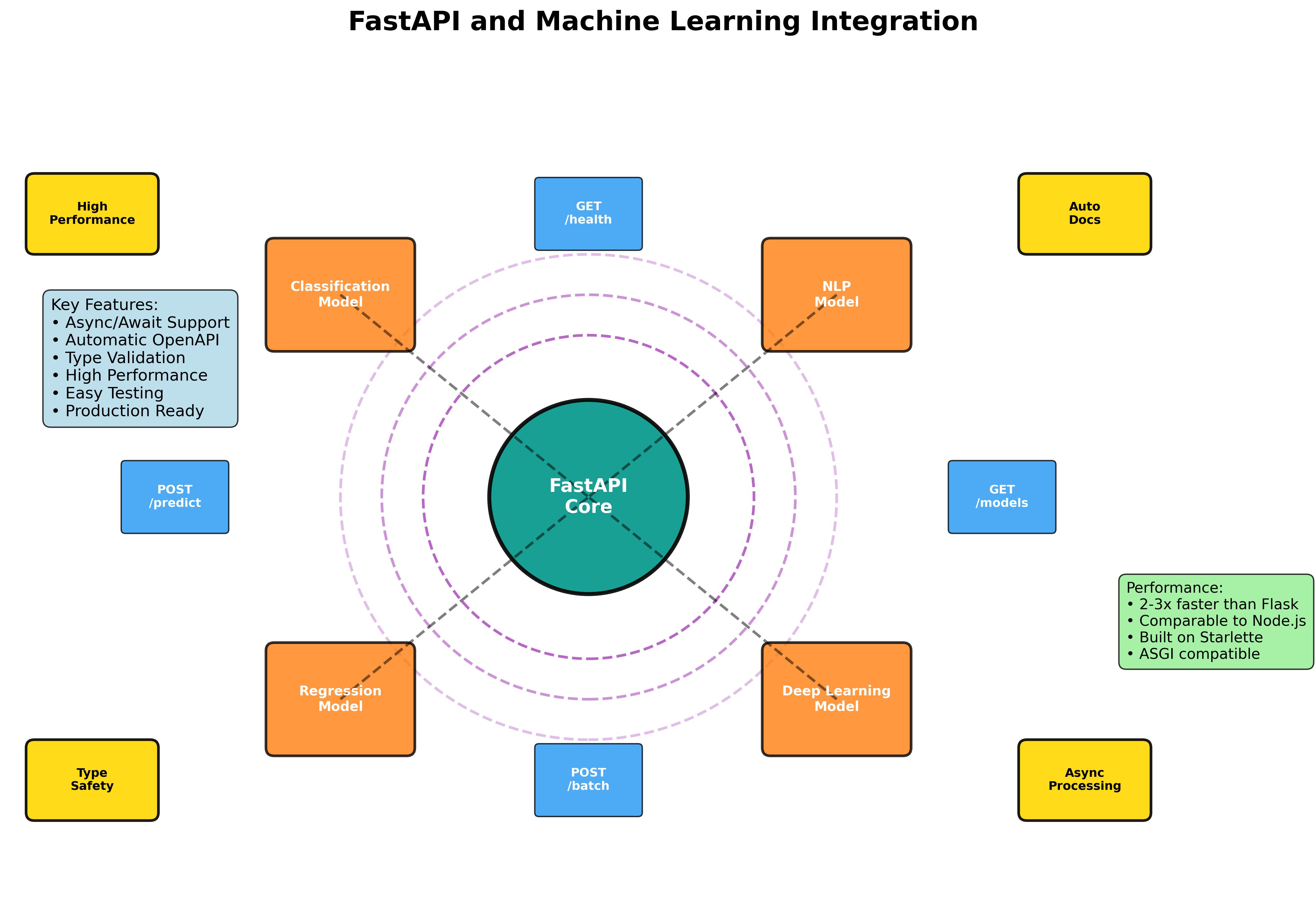
Master the art of building production-ready machine learning APIs with FastAPI. From basic model serving to advanced async processing and containerized deployment.
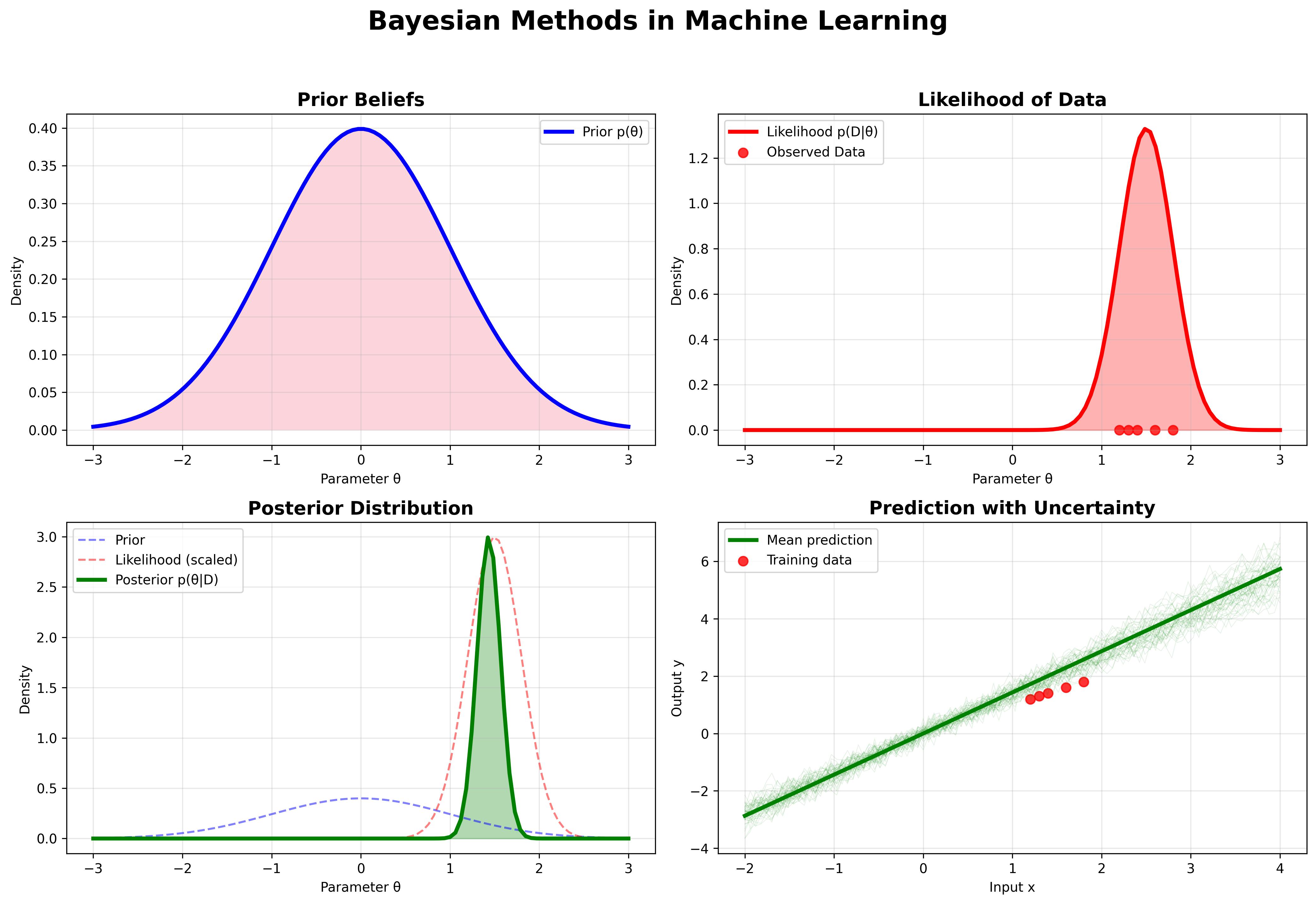
Explore the fundamental principles of Bayesian machine learning, from basic probability theory to advanced applications in modern AI systems.